How to Highlight Duplicates in Google Sheets

When you’re dealing with a lot of data, there may be times when you want to double-check and make sure no duplicates exist—or, conversely, you may want to highlight any duplicates to call attention to them. In that case, there’s a straightforward formula to use in Google Sheets.  

Ready to deepen your knowledge of Google Sheets?

To begin, you'll need your tab open to your spreadsheet. If you’re not already working with your own data set and want to follow along with our examples, make a copy of this template to practice. 

How to highlight duplicates in Google Sheets

Highlighting duplicates in Google Sheets requires conditional formatting using the custom formula =COUNTIF (A:A, A1)>1. Let’s review how to use it.  

TIP: If you’d rather not dive into formulas just yet, you can download an add-on from Google Sheets that will find and highlight duplicates for you.

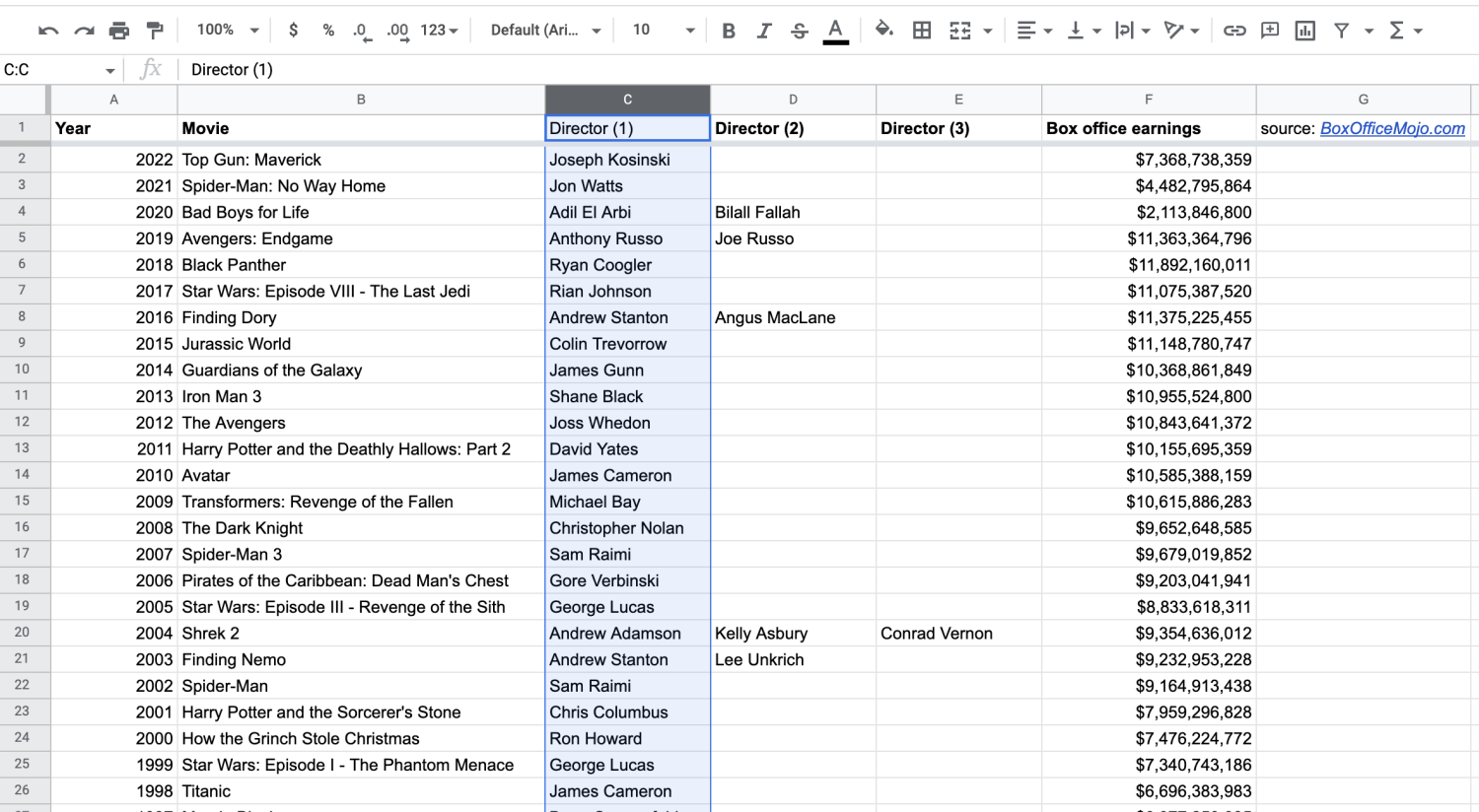
1. Highlight the column you want to find duplicates in.

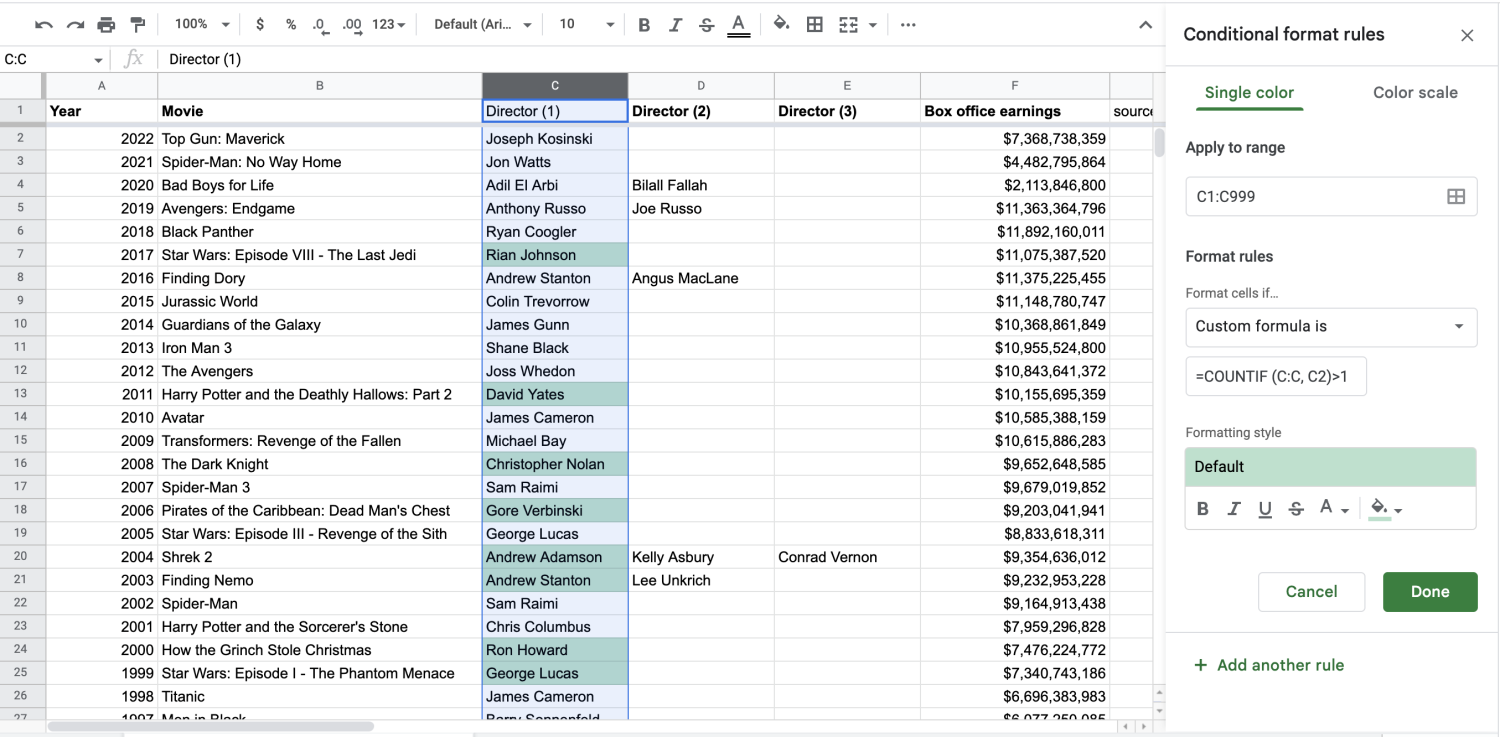
Using our practice sheet, let’s see if there are any duplicates in the Director (1) column.

2. Click 'Format' in the top menu.

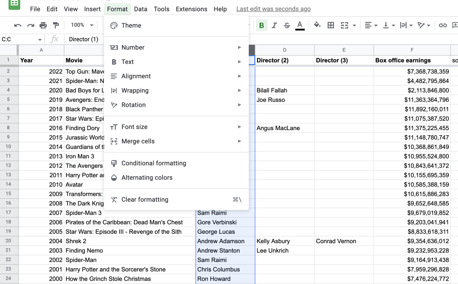
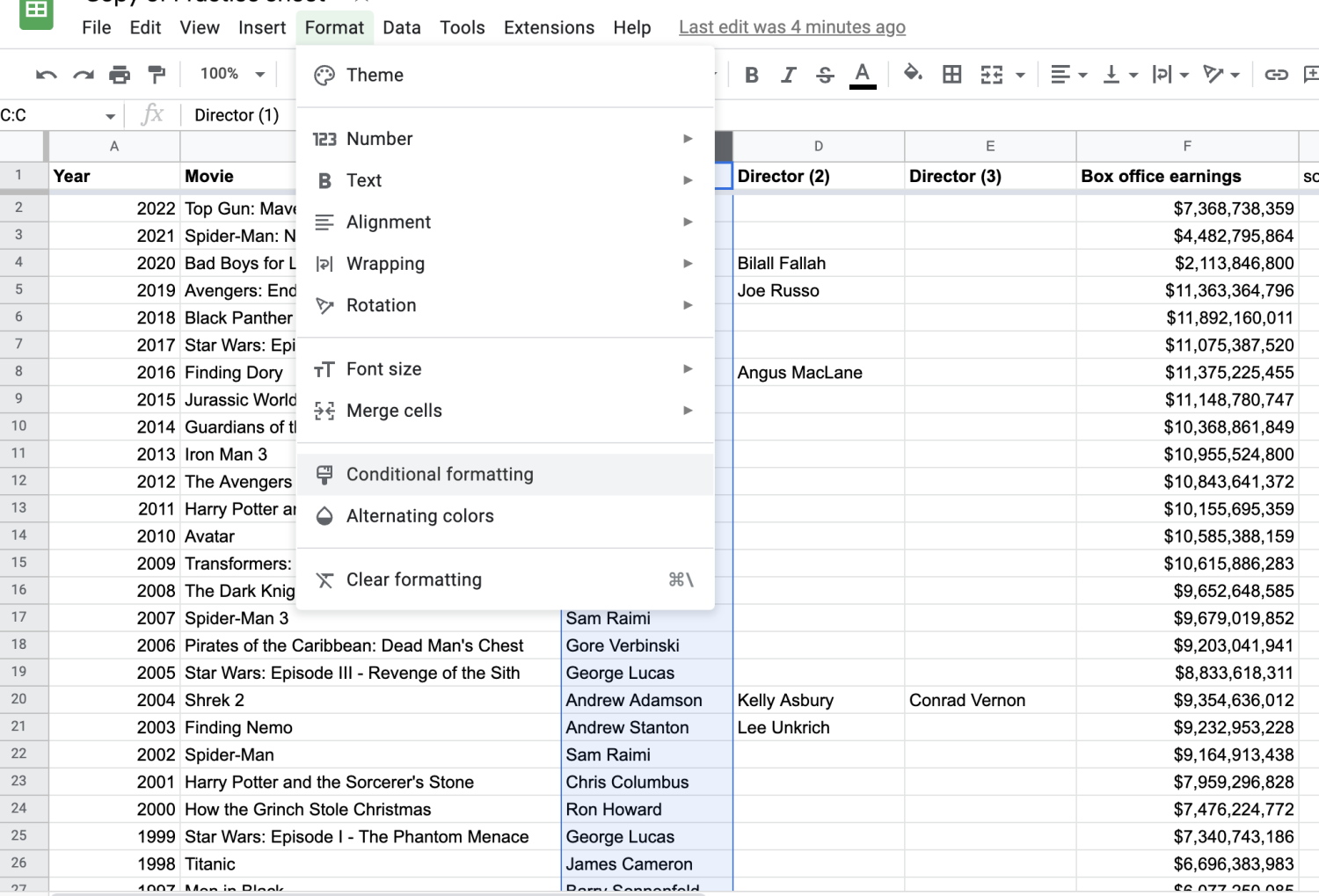
3. Click 'Conditional formatting.'

This will populate a box on the right-hand side of the screen. You’ll see a prompt called “Format cells if…” Click on that and scroll to the bottom. 

Learn more: How to Use Conditional Formatting in Google Sheets

4. In the 'Format cells if' box, click 'Custom formula is.'

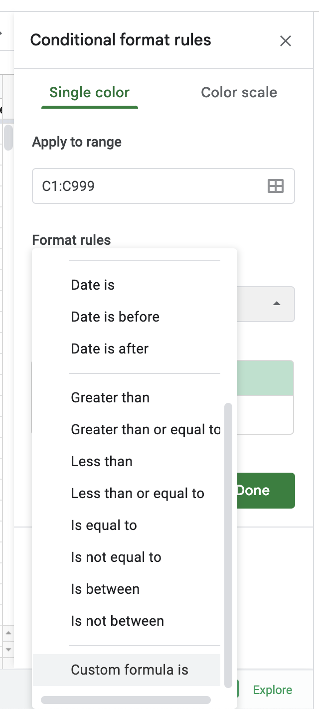
5. Use the COUNTIF formula to find duplicates.

The COUNTIF formula [=COUNTIF (A:A, A1)>1] tells Sheets where to look for duplicates. The information in the parentheses represents the column you want to track and the specific cell you want to start with. The information outside the parentheses states that you want Sheets to count duplicates, or anything appearing more than once (>1). 

Since we’re looking for duplicate directors, we want to adjust the formula to read the C column. Our formula should become =COUNTIF (C:C, C2)>1. You can see how it begins to highlight repeat directors. 

How to count duplicates in multiple columns

Now that you know how to count duplicates in one column, let’s talk about how to adjust the process to count duplicates in multiple columns.

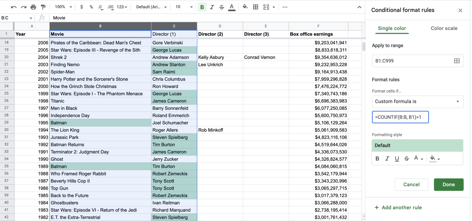
Let’s say you want to check movie titles and directors, so columns B and C in this case. We’ve purposely added an error in the titles column, repeating Batman twice. Clear any previous conditional format rules, and repeat the steps above until you get to the box where you’ll input your custom formula. 

There are now two ways to go about this: 

1. Use 'Apply to range.'

By highlighting the columns you want to check, you’ll automatically tell Apply to range what to concentrate on, but you’ll have to adjust your custom formula to start with the value of that first column and first row. 

For our purposes, we’re looking at columns B and C, so our function should be =COUNTIF(B:B, B1)>1. That tells Sheets to start with B1 and go from there. 

You can adjust the range in Apply to range as needed. Let’s say you were looking at columns B and C, but now you want to include columns B through F. Rather than clear the conditional formatting, highlight your new columns, and start over, you can simply update the “Apply to range” to read “B1:F999.” 

Make sure the syntax of your formula matches the first value. For example, if we want to look at columns C through F now, we’ll update “Apply to range” to “C1:F999” and then make sure the function reads =COUNTIF(C:C, C1)>1. 

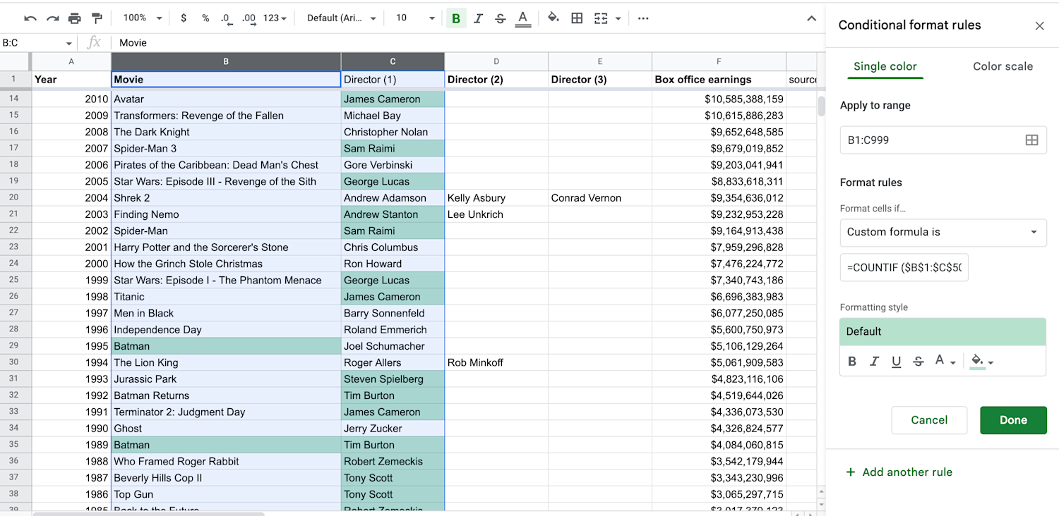
2. Use absolute values. 

Absolute values are a way to specify where Sheets should look for duplicates with the “$” symbol. You’ll need to frame every cell with a “$.” Our function becomes =COUNTIF ($B$1:$C$50, B1)>1. 

How to highlight multiple columns using different colors

Performing the steps we’ve outlined above will highlight your duplicates using one color. But if you have multiple duplicates, you won't be able to see how many of each duplicate you have. 

In that case, you’d want to do a pivot table, which can help you see and better understand the relationship between data.

Explore further

Interested in strengthening your abilities to work with data using Google Sheets? Enroll in the Google Data Analytics Professional Certificate. You’ll learn more about spreadsheets and other key analysis tools. 

Build job-ready skills with a Coursera Plus subscription

Start 7-day free trial

• Get access to 7,000+ learning programs from world-class universities and companies, including Google, Yale, Salesforce, and more
• Try different courses and find your best fit at no additional cost
• Earn certificates for learning programs you complete
• A subscription price of $59/month, cancel anytime

Start 7-day free trial