
How to Add and Subtract a Column in Google Sheets
Learn to use the SUM and MINUS functions to perform a variety of actions in your spreadsheets.
![[Featured image] A person in a blue shirt reviews a Google sheet and works on data visualizations.](https://d3njjcbhbojbot.cloudfront.net/api/utilities/v1/imageproxy/https://images.ctfassets.net/wp1lcwdav1p1/40y5vCZHnvEKNDpJNjfkIv/11ac71e807a7a587c182d0e9e4f17f21/GettyImages-518468392.jpg?w=1500&h=680&q=60&fit=fill&f=faces&fm=jpg&fl=progressive&auto=format%2Ccompress&dpr=1&w=1000)
There are times when it’s helpful to quickly understand the relationship between two or more cells—or an entire column—in Google Sheets. In those cases, you can use functions like SUM (add) or MINUS (subtract) to find the total or difference.
Let’s review how to work with both of these functions.
SUM and MINUS formula
The SUM syntax is:
=SUM(value1, [value2, ...])
value1: The first number, cell, or range to add
value2: (Optional) the second number, cell, or range to add
The MINUS syntax is:
=MINUS (value1, value2)
value1: the number, cell, or range to be subtracted from
value2: the number, cell, or range to subtract
How to SUM in Google Sheets
Ready to deepen your knowledge of Google Sheets?
To begin, you'll need your tab open to your spreadsheet. If you’re not already working with your own data set and want to follow along with our examples, make a copy of this template to practice.

When you’re looking to find the sum total of data in Google Sheets, you can add cells or an entire column together using the SUM function.
1. Choose an empty cell where you’d like the sum to appear.
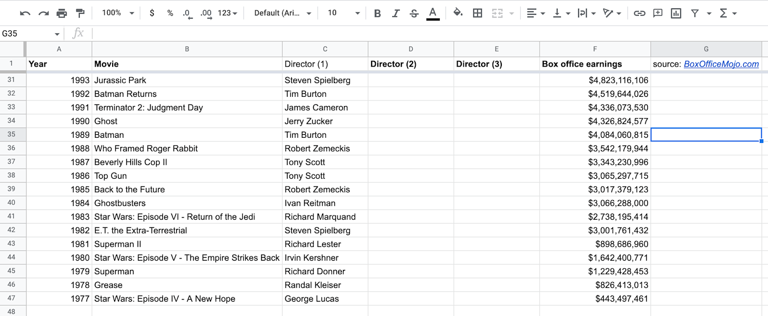
Let’s use SUM to understand more about the column Box Office Earnings in our practice sheet. We could choose a cell at the end of the Box Office Earnings column, or we could choose a cell next to the data we want to add.
2. Use the SUM function to add two cells.
When you begin to type “=SUM” into an empty cell, Google Sheets will automatically display the SUM function =SUM(value1,value2). The comma here tells Sheets to add these values together. Values can be specific cells, numbers, or ranges.
To add two cells, your two values will be the cells you want to total. For example, =SUM(A2, A3) will add cells A2 and A3. Or =SUM(A2, A3, A4) will add cells A2, A3, and A4.
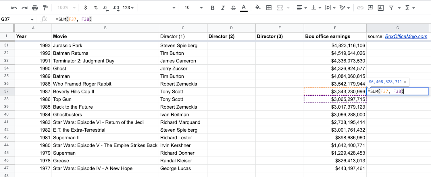
For our practice, let’s have Sheets SUM the movies directed by Tony Scott in the 1980s, so rows F37 and F38. In that case, our function should read =SUM(F37, F38). With that function, we get the total earnings for his 1980s films, Top Gun and Beverly Hills Cop II.

3. Use the SUM function to add a range of cells.
Let’s say you want to find the total for a range of cells (which also works for an entire column). In that case, you’d only need to define one value in you SUM function, and that value will be a range, =SUM(value1). A range is written as two cells separated by a colon, [first cell]:[last cell].
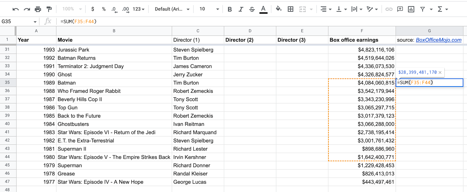
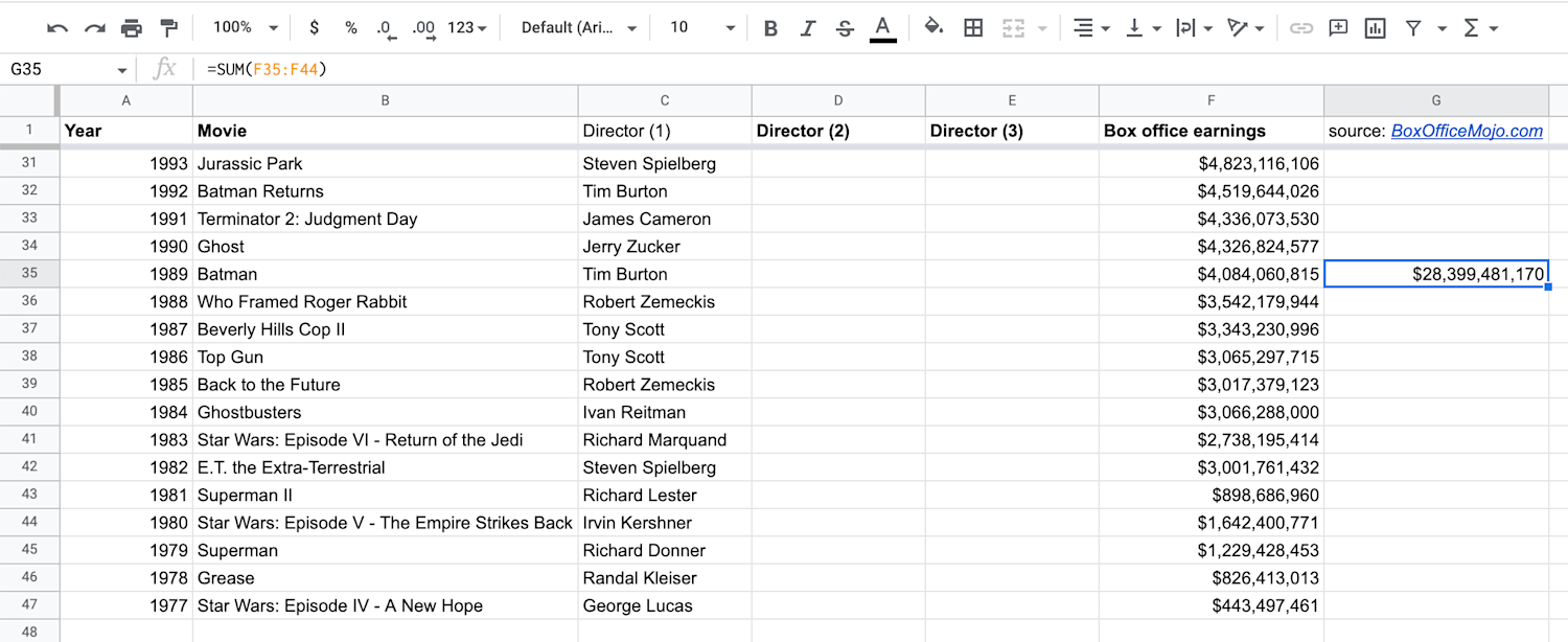
For our practice, let’s add together all movies in the 1980s or F35-44. Our formula should be =SUM(F35:F44).
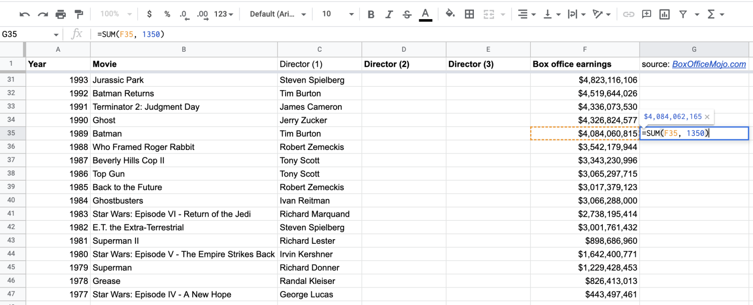
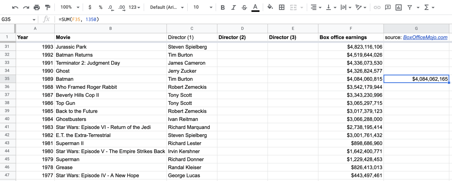
4. Use the SUM function to add a specific number.
If you want to add a specific number to data you’ve accumulated, you can use a number as one of your values.
For example, if you want to find out what an extra $1,350 in ticket sales would add to 1989’s Batman, the function would become =SUM(F35,1350).
How to subtract in Google Sheets
Similar to the SUM function, you can use the MINUS function to figure out the difference between two cells or an entire column.
1. Choose an empty cell where you’d like the difference to appear.
As with SUM, you can choose whichever empty cell makes sense—something beside a row of numbers or at the end of a column of numbers.
2. Use the MINUS function to subtract cells.
When you begin to type “=MINUS” into an empty cell, Google Sheets will automatically populate the MINUS function =MINUS(value1,value2). The comma here once again tells Sheets to subtract these values. Note that the MINUS function can only handle two values, and your values can be specific cells, numbers, or a range.
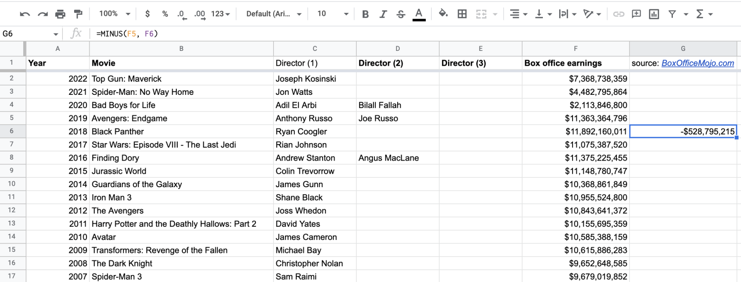
To subtract two cells, your values will be your two cells. For example, let’s say we want to find out how much more Blank Panther grossed compared to Avengers: Endgame. Our function becomes =MINUS(F6, F5) because we know Black Panther (F6) made more and we want to subtract Avengers (F5).
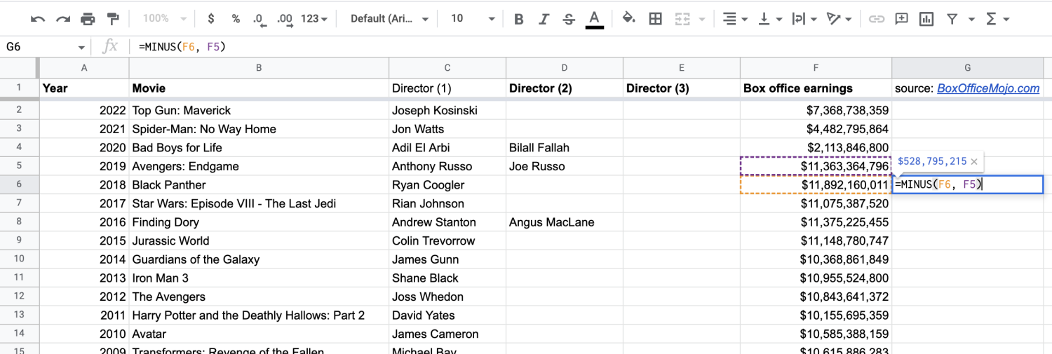

If you subtracted F5 from F6, you’d get the same number, but it should show a negative quality because Avengers didn’t earn as much.
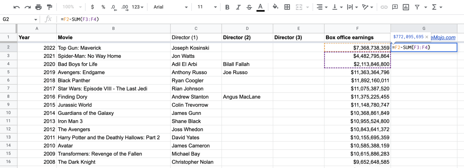
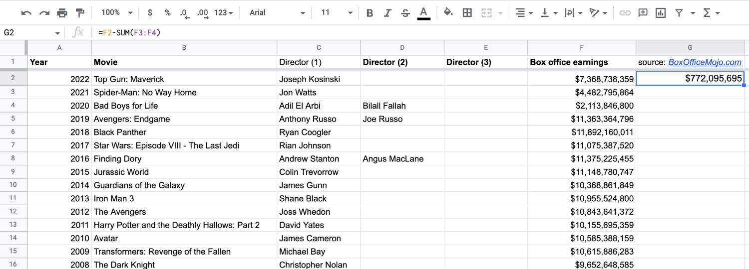
3. Subtract multiple cells from the total of one cell.
If you’d like to subtract multiple cells from the total of one cell, you’ll need to use the subtract formula and the SUM function. (The MINUS function won’t help here because it’s designed to look at the difference between no more than two values.)
The formula to subtract multiple cells from one cell is =value1-SUM(value2,value3). This tells Sheets to add together your second and third values and subtract it from the first.
For example, let's add together Bad Boys for Life and Spider-Man: No Way Home, and subtract them from Top Gun: Maverick. Our formula becomes =F2-SUM(F3:F4).
How to copy the SUM and MINUS functions to an entire column
There may be times when you need to apply the SUM or MINUS functions to an entire column, capturing the total—or difference—of two or more cells for each row. There’s a straightforward way to copy the SUM function and apply it to an entire column.
1. Add the function to your first cell.
Let’s say you want to add columns A and B, to understand the relationship between each row. Start by adding the SUM function to your first cells, A2 and B2. (The steps are the same for the MINUS function.)
2. Double-click the small blue box.
You’ll notice a small blue box appear in the bottom right corner of your highlighted cell. Double-click it to apply the function to the entire column.
Common SUM and MINUS errors and solutions
The issues below most commonly arise when using SUM or MINUS. If you’re not getting the information you want, use the tips below.
#N/A error: The MINUS function can only handle two values, so if you try to add more, such as by subtracting a range, you’ll see #N/A because Sheet was expecting two values (or “two arguments,” as it will explain) and it got more than that.
If the function doesn’t populate an answer or you get “0” as your total: There may be text somewhere in your cells. For instance, Sheets reads currency symbols as text, so adding cells or columns denoting currency ($25 or £100) may create an error. Double-check to make sure you’re adding or subtracting only numerical values.
Clearing one function before using another: If you want to apply a function to an entire column that already has an existing function, you’ll have to first clear that data before Sheets will apply the new function.
Read more: How to Fix Formula Parse Error: Google Sheets
Explore further
Learn more about key data analysis tools, like spreadsheets, by enrolling in the Google Data Analytics Professional Certificate. It’s self-paced, meaning you can learn on your own time, and takes around six months to complete.
Keep reading
Coursera Staff
Editorial Team
Coursera’s editorial team is comprised of highly experienced professional editors, writers, and fact...
This content has been made available for informational purposes only. Learners are advised to conduct additional research to ensure that courses and other credentials pursued meet their personal, professional, and financial goals.