
Using IMPORTRANGE to Reference Another Google Sheet
Learn how to transfer data between Google Sheets and troubleshoot common errors with the IMPORTRANGE function.
![[Featured image] A team reviews data visualizations together at a conference table.](https://d3njjcbhbojbot.cloudfront.net/api/utilities/v1/imageproxy/https://images.ctfassets.net/wp1lcwdav1p1/69Lyp4NkgwJPKy9SDGIafZ/a8d9fc256fc622f63a2f6c6e2fb4824c/GettyImages-981250802.jpg?w=1500&h=680&q=60&fit=fill&f=faces&fm=jpg&fl=progressive&auto=format%2Ccompress&dpr=1&w=1000)
IMPORTRANGE enables you to replicate data from one Google Sheet to another. When you use this function, data on the imported sheet will automatically update to reflect the data in the original spreadsheet, making it a useful way to reference up-to-date data from a separate Google Sheet without having to keep multiple spreadsheets open.
The syntax for IMPORTRANGE is =IMPORTRANGE(spreadsheet_url, range_string).
By the end of this tutorial, you will be able to transfer data from another Google Sheet using the IMPORTRANGE function.
IMPORTRANGE formula
The IMPORTRANGE syntax is:
=IMPORTRANGE(spreadsheet_url, range_string)
Here’s what those inputs refer to:
spreadsheet_url: The URL of the original spreadsheet with the data you want to bring into your new sheet
range_string: The area in the original spreadsheet containing the data you want to bring into your new sheet
How to use IMPORTRANGE
Ready to deepen your knowledge of Google Sheets?
To begin, you'll need your tab open to your spreadsheet. If you’re not already working with your own data set and want to follow along with our examples, make a copy of this template to practice.

For this function, you’ll need two spreadsheets open: one spreadsheet that houses your original data and a second destination sheet where you want to import that original data. If you’re following along with our template, you’ll want to have that spreadsheet open in addition to a new blank spreadsheet.
Let’s take a closer look at how to identify your inputs and use IMPORTRANGE in Google Sheets.
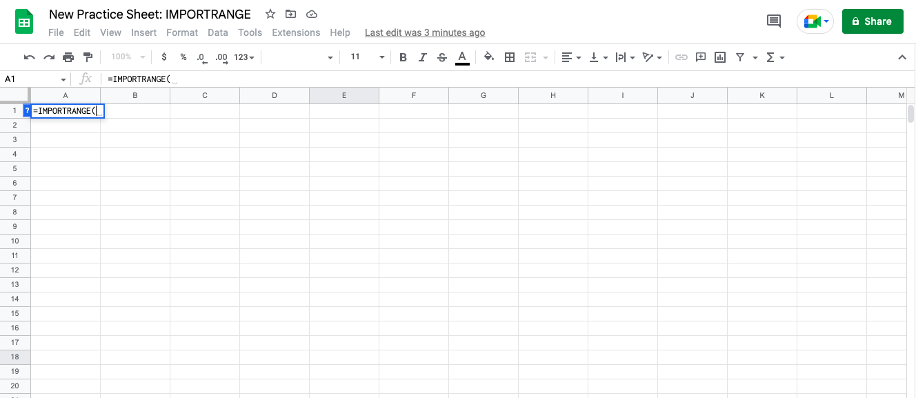
1. In your new spreadsheet, click on the top-leftmost cell in the area where you want the imported data to appear.
The cell where you type the IMPORTRANGE function will become the top-leftmost cell in your imported range. There, start your function with =IMPORTRANGE(.
In my practice sheet, I’ll start my function in cell A1.
2. Copy the URL of the spreadsheet containing the data you want to import.
The first input, the spreadsheet URL, refers to the URL of the original spreadsheet that houses your data. To copy the URL, go to your original spreadsheet, highlight the URL in full, right click, and select ‘Copy.’
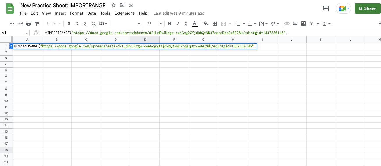
Then, return to your new spreadsheet. Paste the URL into your function surrounded by quotation marks (").
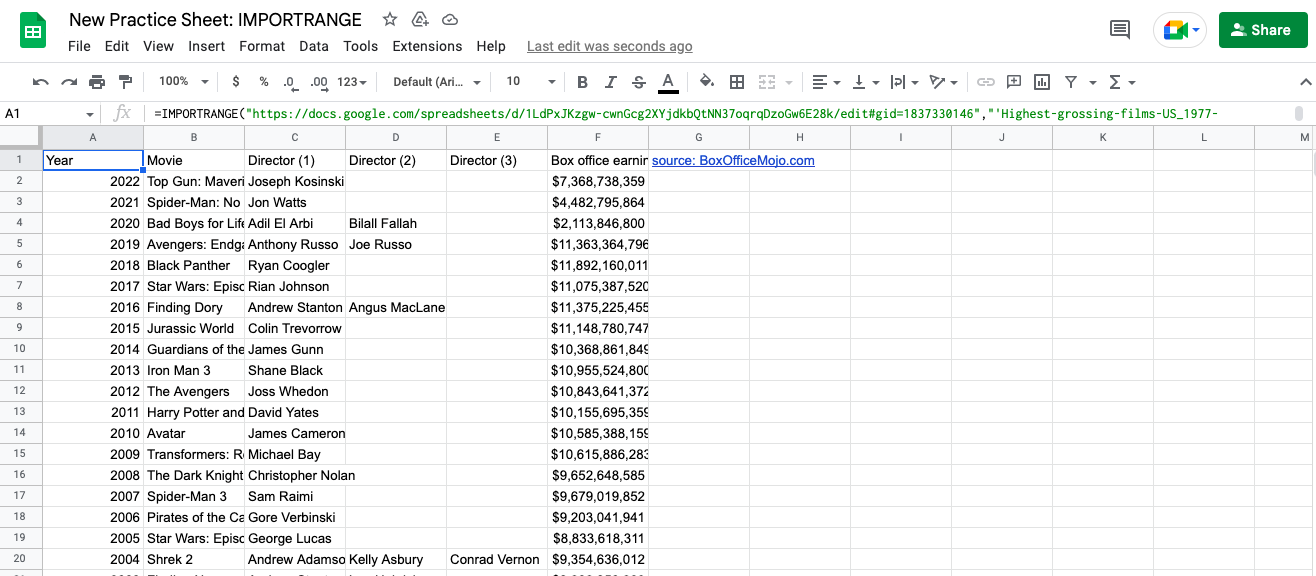
In my Practice Sheet, my function now reads =IMPORTRANGE("https://docs.google.com/spreadsheets/d/1LdPxJKzgw-cwnGcg2XYjdkbQtNN37oqrqDzoGw6E28k/edit#gid=1837330146",.
3. Identify the range string in your original spreadsheet.
The range string is the area in the original spreadsheet containing the data you want to bring into your new sheet.
The format for the range string is SheetName![top-leftmost cell]:[bottom-rightmost cell]. Here are some points to keep in mind when you’re figuring out your range string:
If your sheet name contains spaces or numbers, put the name in single quotes (').
If you don’t include a sheet name in the range string, this function will automatically import data from the first sheet (tab) in your spreadsheet (workbook).
Your range can be as small as a single cell. If you only want to import one cell, simply cut the range string off before the colon to read SheetName!Cell.
Write the range string in your function, surrounded by quotation marks (").
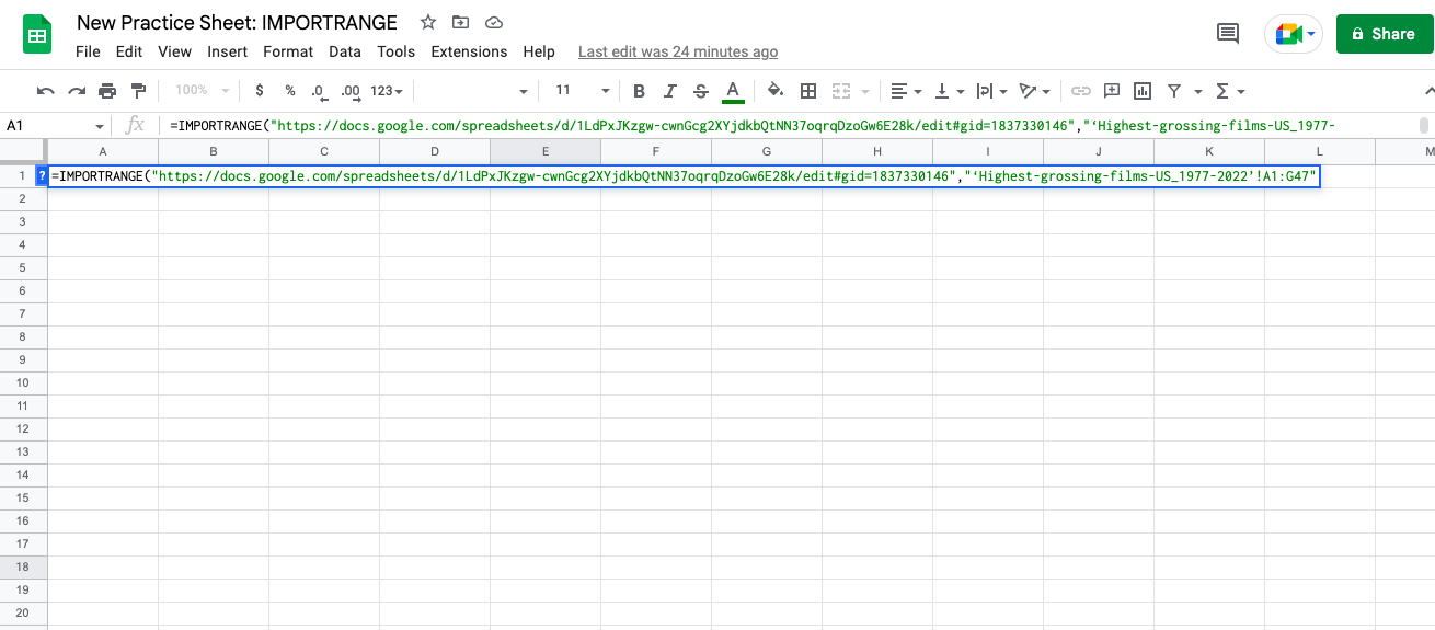
In my Practice Sheet, I’m importing data from the sheet named Highest-grossing-films-US_1977-2022. The top-leftmost cell with my data is A1, and the bottom-rightmost cell is G47. This makes my range string 'Highest-grossing-films-US_1977-2022'!A1:G47.
Now, my function reads =IMPORTRANGE("https://docs.google.com/spreadsheets/d/1LdPxJKzgw-cwnGcg2XYjdkbQtNN37oqrqDzoGw6E28k/edit#gid=1837330146","'Highest-grossing-films-US_1977-2022'!A1:G47".
4. End your function with a closing parenthesis ) and hit enter.
The first time you try importing this data into your new spreadsheet, you’ll get an error message, #REF! This is expected at this point and pertains to sharing permissions.
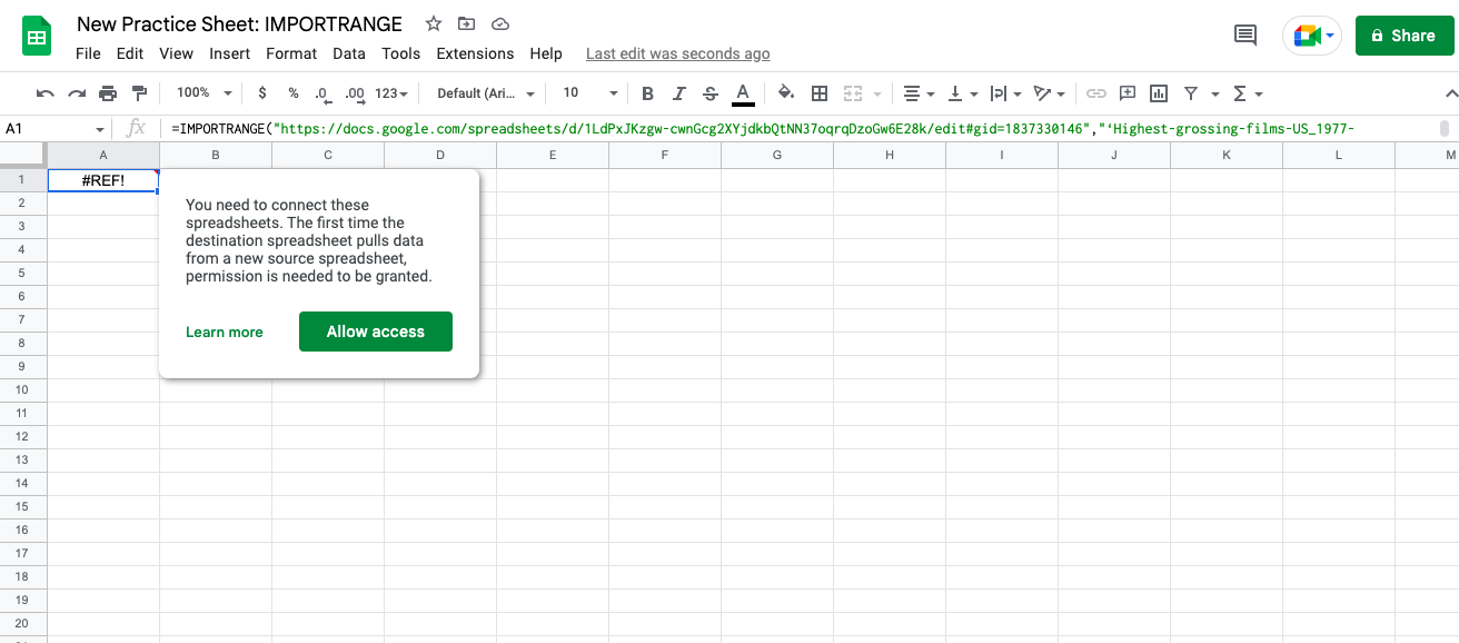
5. Select 'Allow access' to finish importing your data.
Even though your IMPORTRANGE function will still appear if you select the cell you typed the function into, your new spreadsheet will now show a copy of the data from your original spreadsheet.
How to reference another sheet within the same spreadsheet
If you want to import data to a new spot within the same spreadsheet—either on the same tab as your original data or a new one—you can use a simplified formula rather than the IMPORTRANGE function. You just need to type an equal sign and the range for the original data in the top-leftmost cell where you want your replicated data to appear:
='SheetName'![top-leftmost cell]:'SheetName'![bottom-rightmost cell]
If you only want to replicate a single cell, you only need to include that cell in your formula:
='SheetName'!Cell
If your referenced cell appears on the same sheet as your original data, you don’t need to include the sheet name.
IMPORTRANGE limitations and alternatives
IMPORTRANGE replicates data from one spreadsheet onto another and will automatically update the imported data as you add, delete, or otherwise manipulate the original data set. However, when you use IMPORTRANGE, you’ll notice two limitations: (1) you cannot manipulate your imported data, and (2) the formatting from your original sheet will not automatically carry over.
Let’s take a look at how you can work around these limitations.
Working with imported data
While you can perform some tasks with your imported data, such as filtering and performing calculations and functions, you cannot directly change your imported data, such as editing text and sorting.
If you’d like to be able to directly work with your imported data in your new spreadsheet, one way to do that would be to copy your imported data onto a new tab. Here’s how:
Start by highlighting the imported range and copying the data.
Make a new tab in your spreadsheet.
Highlight the first cell in your new tab.
Go to Edit in the top menu. Then, go to Paste special > Values only.
Your imported data will paste as text that you can work with directly.
However, keep in mind that these pasted values won’t automatically update to align with the original spreadsheet. You’ll need to repeat this process each time your original data set is updated.
Formatting imported data
IMPORTRANGE will not import formatting, only the contents of the cells. However, you can manually copy and paste formatting from your original spreadsheet onto your new one. Here’s how:
In your original spreadsheet, highlight the cells in your source range and copy.
In your new spreadsheet, highlight the imported range area.
Go to Edit in the top menu. Then, go to Paste Special > Format only.
The format from your original spreadsheet will paste onto your imported data.
Unfortunately, you cannot paste column widths from one sheet to another, but you can manually resize cells on your new sheet without impacting the IMPORTRANGE function.
Common errors and solutions
If you don’t use the IMPORTRANGE function accurately, you’ll get a formula parse error. Here are some common error messages associated with IMPORTRANGE and suggestions for how you can troubleshoot them.
#ERROR!: This error typically indicates an issue with your syntax. Make sure you’ve written each input correctly and used proper punctuation, including quotation marks around the spreadsheet URL and range string, and have properly formatted your range string.
#REF!: This error typically appears in two instances: (1) when you first import your data and need to allow sharing permissions, and (2) if you try to manipulate any cells within your imported range. In the first scenario, select ‘Allow access’ to import your data. In the second scenario, undo your attempt to manipulate the cells within the imported range. Then, see the above workaround for working with your imported data.
Read more: How to Fix Formula Parse Error: Google Sheets
Keep learning
Interested in strengthening your abilities to work with data using Google Sheets? Enroll in the Google Data Analytics Professional Certificate. You’ll learn more about spreadsheets and other key analysis tools.
Keep reading
Coursera Staff
Editorial Team
Coursera’s editorial team is comprised of highly experienced professional editors, writers, and fact...
This content has been made available for informational purposes only. Learners are advised to conduct additional research to ensure that courses and other credentials pursued meet their personal, professional, and financial goals.